Lab Report | 2D Image Filtering

Lab Report | 2D Image Filtering

This second lab report takes interest in the application of 2D filtering on grayscale images.

Image filtering is the removal of certain characteristics of an image. It is used to reduce noise, enhance edges, highlight certain features, and smooth an image.

In this lab, we will focus on the filtering of spatial frequencies in the frequency domain using the Discrete Cosine Transform (DCT).

The DCT is a Fourier-related transform similar to the discrete Fourier transform (DFT), but using only real numbers. It is equivalent to the DFT of roughly twice the length, operating on real data with even symmetry (since the Fourier transform of a real and even function is real and even), where in some variants the input and/or output data are shifted by half a sample. There are eight standard DCT variants, of which four are common.

1. Computing the 2D-DCT and 2D-IDCT

The first step is to compute the 2D-DCT of the image. The DCT is a linear transformation that maps a vector of pixel values to a vector of frequency coefficients.

Here’s the result of the DCT on lenna.png, as well as the inverse DCT:

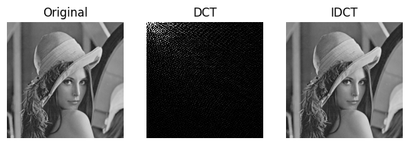
Analysis:

• The lower frequencies define the global shapes of the image, while the higher frequencies define the details of the image. The higher frequencies are more sparse because the image is mostly made of low frequencies with some patterns of high frequencies.
• The inverse DCT restores the original image as the DCT is a lossless, reversible transformation.

---

2. Applying Low Pass Filtering

Low Pass filtering in the frequency domain is equivalent to removing high frequencies from the image. This is done by setting the high frequency coefficients to zero:

def low_pass(image, fc):
    lp = np.zeros(image.shape)
    lp[:fc, :fc] = image[:fc, :fc]
    return lp

This code snippet sets the high frequency coefficients to zero from the cutting frequency fc and up, and returns the resulting image.

Here’s the result of the low pass filtering on lenna.png:

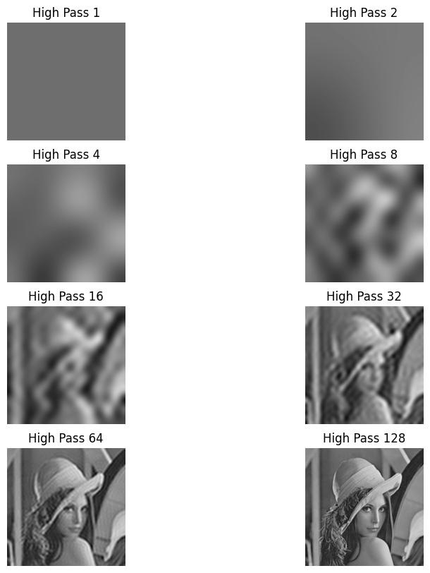
and the result on baboon.png:

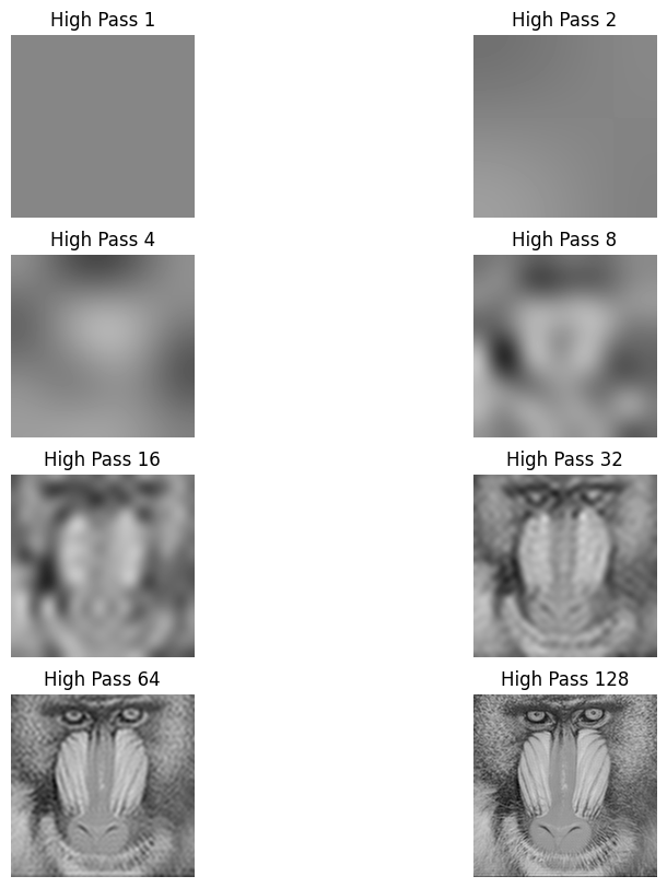
Analysis :

• The low pass filtering removes the high frequencies from the image, which are the details of the image. The resulting image is blurred and the details are lost.

---

3. Applying High Pass Filtering

Inverse to low pass filtering, high pass filtering in the frequency domain is equivalent to removing low frequencies from the image. This is done by setting the values in the top left corner of the frequency domain to zero:

def high_pass(image, fc):
    hp = image.copy()
    hp[:fc, :fc] = 0
    hp[0,0] = image[0,0]
    return hp 

This code snippet sets the low frequency coefficients to zero from the cutting frequency fc and down, and returns the resulting image.

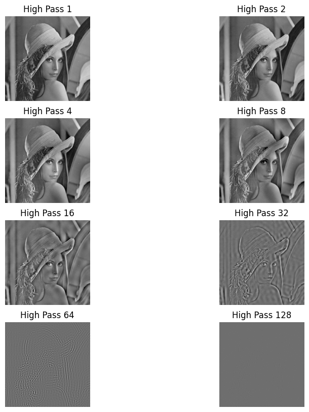
Here’s the result of the high pass filtering on lenna.png:

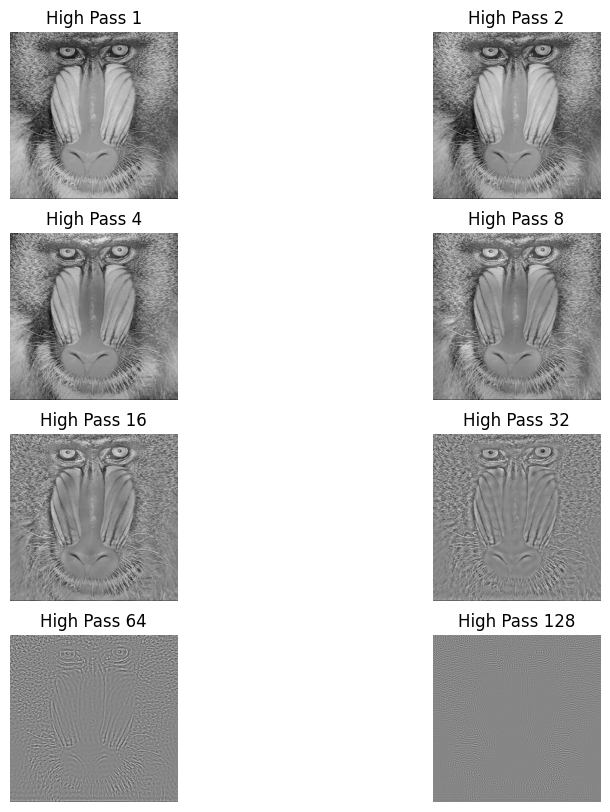
and the result on baboon.png:

Analysis :

• The high pass filtering removes the low frequencies from the image, which are the global shapes of the image. The resulting image is the details of the image.
• We also notice that High Pass filtering tends to keep the edges of the image.

---

4. Mixing High Pass and Low Pass of different images

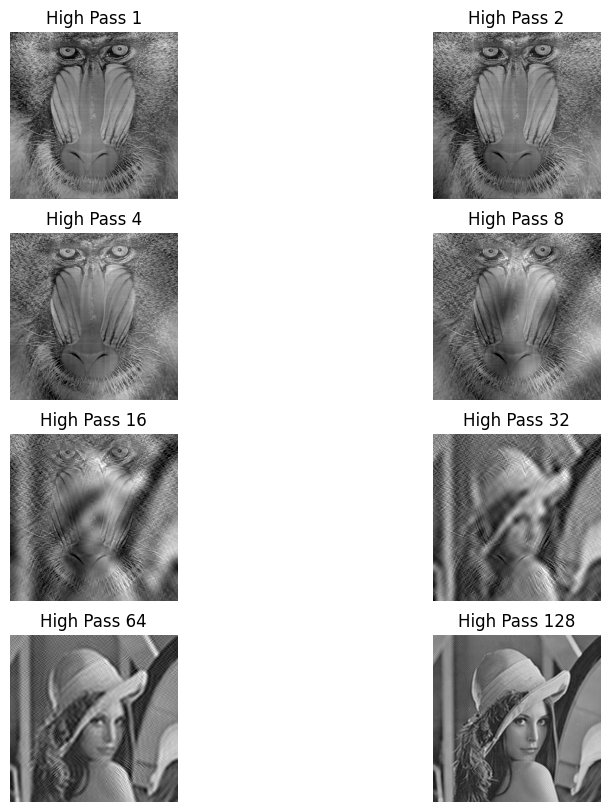
We can also mix the high pass and low pass filtering of different images. Here’s the result of the low pass filtering of lenna.png and the high pass filtering of baboon.png:

Analysis :

• The resulting image is a mix of the details of lenna.png and the edges of baboon.png.

---